Multiple compartments

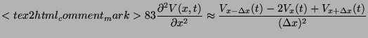
In the trapezoidal scheme the following rule is used to spatially discretize the cylindrical cable equation:

$$<tex2html_comment_mark>83 \frac{\partial^2V(x,t)}{\partial x^2} \approx \frac{V_{x - \Delta x}(t) - 2 V_x(t) + V_{x + \Delta x}(t)}{(\Delta x) ^2}$$ (1.12)

This scheme splits up a single cable in multiple compartments and is second-order accurate in space if the discretization length is kept constant (use the Taylor series to prove this: take the sum of a Taylor expansion for $V(x + \Delta x)$ and $V(x - \Delta x)$ and see what happens). It is used by most popular neuro-biological simulation packages to discretize dendritic trees (however with a non constant discretization length, which makes the rule first order accurate).

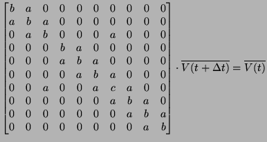
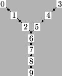
If this scheme is combined with an explicit numerical scheme like the exponential Euler, all the resulting equations are self contained and can be solved in isolation. However if this scheme is combined with an implicit numerical scheme like the backward-Euler, the numerator of the right-hand side couples the neighboring compartments to each other. it gives rise to a system of coupled finite-difference equations. If you choose the trapezoidal rule for time discretization, the method is called a Crank-Nicolson. For a linear cable the coefficients of this system can be arranged in a tridiagonal matrix such that it can be solved in linear time. For branched morphologies the matrix is still symmetric (not tridiagonal however), and it can still be solved in linear time. The arrangement of the equations is done with Hines numbering (a special kind of minimum degree algorithm, see[7]), and the solution can be obtained with Gaussian elimination without pivoting[8,7]. This operation scales with the number of equations in the system and as such it can be considered to be a fast solution for this system. Figure 1.2.2 gives an example morphology with the corresponding matrix structure. The text below the figure gives more explanation about how to solve the system of equations.

NOTE: Without extensions these schemes cannot be applied to gap junctions, since gap junctions give rise to looped electrical circuits such that the matrix containing the cable equations, cannot be solved with Gaussian elimination without pivoting.

Figure: Resulting matrix structure after applying an implicit numerical scheme to the shown morphology. The numbers in the figure correspond to the rows in the matrix and come from one possible (Hines) numbering scheme[7]. The system can easily be solved by sweeping through the equations twice: the first sweep eliminates all the coefficients below the main diagonal and results in the decoupling of the last equation such that it can be solved in isolation. Then the second sweep starts by substituting the last unknown in the second last equation, such that this equation can be solved too. Continuing this process upwards solves the complete system. (Application of an explicit numerical scheme to this morphology would result in a matrix with only coefficients on the main diagonal. Of course in such a system all equations can be solved in isolation.)

$\begin{bmatrix} b & a & 0 & 0 & 0 & 0 & 0 & 0 & 0 & 0 \\ a & b & a & 0 & 0 & ... ... \\ \end{bmatrix}\cdot \overline{V(t + \Delta t)} = \overline{V(t)} \nonumber$